Week 6: Campaign Expenditure #
Monday, October 14, 2024
21 Days until Presidential Election
We are now less than a month away from election day! It means a lot that you’ve followed along this far. Thank you! This week, we will be considering how campaign advertisement expenditure can play a role in election outcomes. In the 2020 Presidential Elections, I remember one day receiving over 20 campaign flyers and virtually the only ads aired on television being political. I thought that, if forecasters could take a metric of campaign mail count in my suburban Atlanta district, they’d probably have a more accurate model. I cannot monitor the ads in Georgia as closely as I did in the last election because I’m in college now, but I hope to at least involve available data on campaign ad expenditure into my model.
Campaign Ads and Messaging #
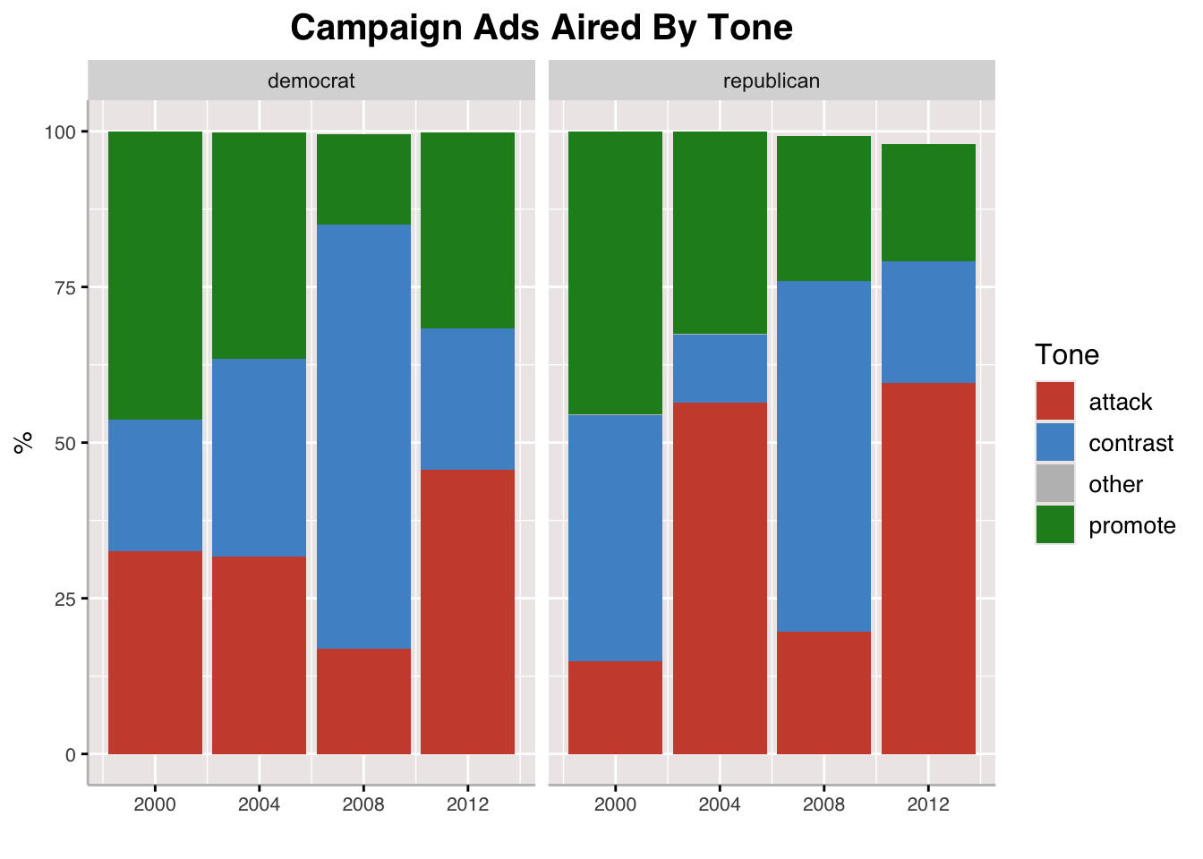
Above, we see a chart presenting the tone of campaign ads by party and by election cycle. We see that across cycles, Democrats tend to not make the majority of their ads with an attacking tone, but in 2004 and 2012, Republicans did just that. Overall, there is no clear trend as to the tone of campaign ads over time, and I would argue that it depends heavily on the candidates running and their style of campaigning.
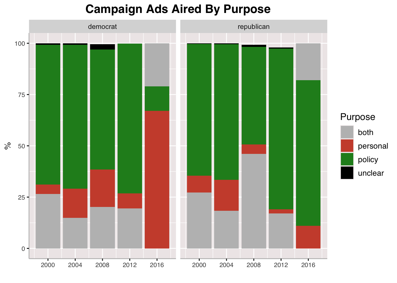
We also see a visualization of of the purpose of campaign ads by party and by presidential election year. Most of the time, we see that policy ads are the most common across parties and across cycles, except for ads by Democrats in 2016. Across most election cycles, it seems that Democrats field more personal ads than Republicans, and this difference can be marginal or staggering like it was in 2016.
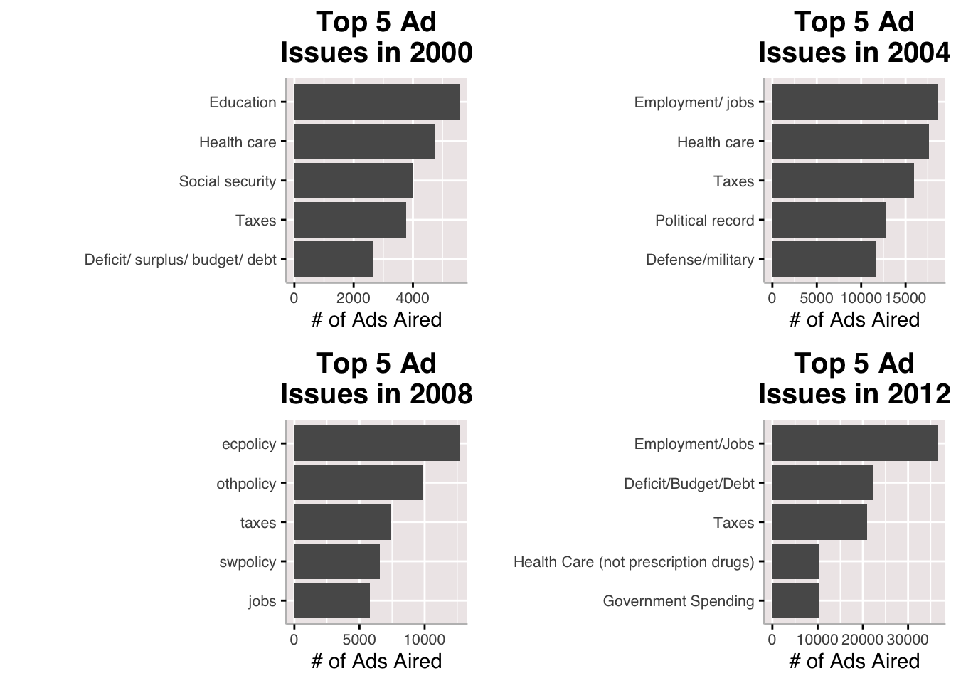
Here, we can take a look at the issues most frequently mentioned in campaign ads across elections from 2000-2012. In addition to there being more ads in general as time goes on, we see a notable changed in the issues that are mentioned in ads between cycles. The one issue that stays across all cycles is taxes and jobs/employment seems pretty sticky as well.
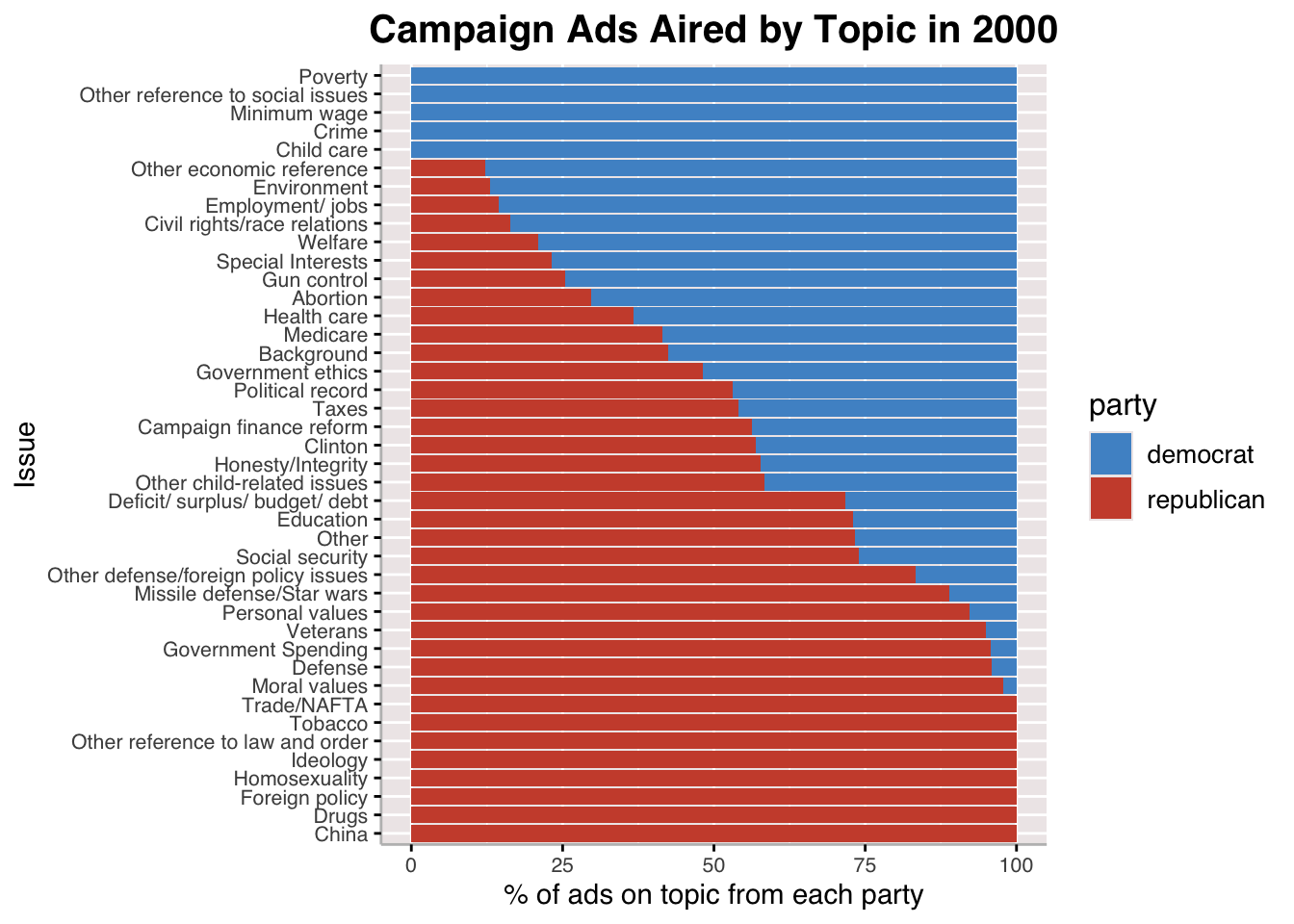
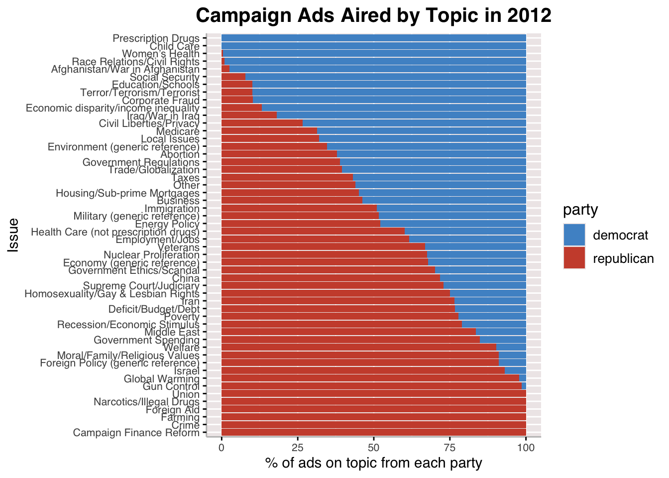
Going into the party split for campaign ads for 2000 and 2012, we see notable differences in the topics for which parties choose to air ads. One thing I find interesting is that, in 2000, Democrats did not touch homosexuality as a topic for campaign ads, and Republicans wre the only ones to air ads on the issue, presumably against it. By 2012, more Democratic ads on homosexuality appeared and the name of the issue changed to a split between Moral/Family/Religious values (for which there were more Republican ads) and Homosexuality/Gay & Lesbian Rights.
Those issues which both parties pretty evenly air ads on are also very similar to the issues observed in the first plot, which shows the most frequently mentioned issues in campaign ads regardless of party and across election cycles. Taxes, healthcare, and deficit are among them.
Campaign Expenditure Model #
| Model 1 | Model 2 | |
|---|---|---|
| (Intercept) | 46.808 | −23.093 |
| (0.771) | (7.160) | |
| contribution_receipt_amount | 0.0000002 | |
| (3e−08) | ||
| log(contribution_receipt_amount) | 4.659 | |
| (0.460) | ||
| Num.Obs. | 200 | 200 |
| R2 | 0.168 | 0.341 |
| R2 Adj. | 0.163 | 0.338 |
| AIC | 1476.7 | 1430.1 |
| BIC | 1486.6 | 1439.9 |
| Log.Lik. | −735.367 | −712.027 |
| F | 39.886 | 102.423 |
| RMSE | 9.56 | 8.51 |
The model summary we see here is a linear regression for Democratic campaign spending and the Democratic two-party vote share. Model 1 refers to treating campaign expenditure as an unmodified variable while Model 2 applies a log transformation to better understand the relationship between the two variables. We see that, in the context of this linear regression, campaign expenditure for Democrats has a positive impact on their two party vote share. This motivates my inclusion of campaign expenditure data into the model I use to predict the outcome of the 2024 elections.
Bayesianism #
##
## SAMPLING FOR MODEL 'anon_model' NOW (CHAIN 1).
## Chain 1:
## Chain 1: Gradient evaluation took 9.5e-05 seconds
## Chain 1: 1000 transitions using 10 leapfrog steps per transition would take 0.95 seconds.
## Chain 1: Adjust your expectations accordingly!
## Chain 1:
## Chain 1:
## Chain 1: Iteration:    1 / 4000 [  0%]  (Warmup)
## Chain 1: Iteration:  400 / 4000 [ 10%]  (Warmup)
## Chain 1: Iteration:  800 / 4000 [ 20%]  (Warmup)
## Chain 1: Iteration: 1001 / 4000 [ 25%]  (Sampling)
## Chain 1: Iteration: 1400 / 4000 [ 35%]  (Sampling)
## Chain 1: Iteration: 1800 / 4000 [ 45%]  (Sampling)
## Chain 1: Iteration: 2200 / 4000 [ 55%]  (Sampling)
## Chain 1: Iteration: 2600 / 4000 [ 65%]  (Sampling)
## Chain 1: Iteration: 3000 / 4000 [ 75%]  (Sampling)
## Chain 1: Iteration: 3400 / 4000 [ 85%]  (Sampling)
## Chain 1: Iteration: 3800 / 4000 [ 95%]  (Sampling)
## Chain 1: Iteration: 4000 / 4000 [100%]  (Sampling)
## Chain 1:
## Chain 1:  Elapsed Time: 1.448 seconds (Warm-up)
## Chain 1:                4.447 seconds (Sampling)
## Chain 1:                5.895 seconds (Total)
## Chain 1:
##
## SAMPLING FOR MODEL 'anon_model' NOW (CHAIN 2).
## Chain 2:
## Chain 2: Gradient evaluation took 1.6e-05 seconds
## Chain 2: 1000 transitions using 10 leapfrog steps per transition would take 0.16 seconds.
## Chain 2: Adjust your expectations accordingly!
## Chain 2:
## Chain 2:
## Chain 2: Iteration:    1 / 4000 [  0%]  (Warmup)
## Chain 2: Iteration:  400 / 4000 [ 10%]  (Warmup)
## Chain 2: Iteration:  800 / 4000 [ 20%]  (Warmup)
## Chain 2: Iteration: 1001 / 4000 [ 25%]  (Sampling)
## Chain 2: Iteration: 1400 / 4000 [ 35%]  (Sampling)
## Chain 2: Iteration: 1800 / 4000 [ 45%]  (Sampling)
## Chain 2: Iteration: 2200 / 4000 [ 55%]  (Sampling)
## Chain 2: Iteration: 2600 / 4000 [ 65%]  (Sampling)
## Chain 2: Iteration: 3000 / 4000 [ 75%]  (Sampling)
## Chain 2: Iteration: 3400 / 4000 [ 85%]  (Sampling)
## Chain 2: Iteration: 3800 / 4000 [ 95%]  (Sampling)
## Chain 2: Iteration: 4000 / 4000 [100%]  (Sampling)
## Chain 2:
## Chain 2:  Elapsed Time: 1.371 seconds (Warm-up)
## Chain 2:                4.142 seconds (Sampling)
## Chain 2:                5.513 seconds (Total)
## Chain 2:
##
## SAMPLING FOR MODEL 'anon_model' NOW (CHAIN 3).
## Chain 3:
## Chain 3: Gradient evaluation took 1.5e-05 seconds
## Chain 3: 1000 transitions using 10 leapfrog steps per transition would take 0.15 seconds.
## Chain 3: Adjust your expectations accordingly!
## Chain 3:
## Chain 3:
## Chain 3: Iteration:    1 / 4000 [  0%]  (Warmup)
## Chain 3: Iteration:  400 / 4000 [ 10%]  (Warmup)
## Chain 3: Iteration:  800 / 4000 [ 20%]  (Warmup)
## Chain 3: Iteration: 1001 / 4000 [ 25%]  (Sampling)
## Chain 3: Iteration: 1400 / 4000 [ 35%]  (Sampling)
## Chain 3: Iteration: 1800 / 4000 [ 45%]  (Sampling)
## Chain 3: Iteration: 2200 / 4000 [ 55%]  (Sampling)
## Chain 3: Iteration: 2600 / 4000 [ 65%]  (Sampling)
## Chain 3: Iteration: 3000 / 4000 [ 75%]  (Sampling)
## Chain 3: Iteration: 3400 / 4000 [ 85%]  (Sampling)
## Chain 3: Iteration: 3800 / 4000 [ 95%]  (Sampling)
## Chain 3: Iteration: 4000 / 4000 [100%]  (Sampling)
## Chain 3:
## Chain 3:  Elapsed Time: 1.242 seconds (Warm-up)
## Chain 3:                3.81 seconds (Sampling)
## Chain 3:                5.052 seconds (Total)
## Chain 3:
##
## SAMPLING FOR MODEL 'anon_model' NOW (CHAIN 4).
## Chain 4:
## Chain 4: Gradient evaluation took 1.9e-05 seconds
## Chain 4: 1000 transitions using 10 leapfrog steps per transition would take 0.19 seconds.
## Chain 4: Adjust your expectations accordingly!
## Chain 4:
## Chain 4:
## Chain 4: Iteration:    1 / 4000 [  0%]  (Warmup)
## Chain 4: Iteration:  400 / 4000 [ 10%]  (Warmup)
## Chain 4: Iteration:  800 / 4000 [ 20%]  (Warmup)
## Chain 4: Iteration: 1001 / 4000 [ 25%]  (Sampling)
## Chain 4: Iteration: 1400 / 4000 [ 35%]  (Sampling)
## Chain 4: Iteration: 1800 / 4000 [ 45%]  (Sampling)
## Chain 4: Iteration: 2200 / 4000 [ 55%]  (Sampling)
## Chain 4: Iteration: 2600 / 4000 [ 65%]  (Sampling)
## Chain 4: Iteration: 3000 / 4000 [ 75%]  (Sampling)
## Chain 4: Iteration: 3400 / 4000 [ 85%]  (Sampling)
## Chain 4: Iteration: 3800 / 4000 [ 95%]  (Sampling)
## Chain 4: Iteration: 4000 / 4000 [100%]  (Sampling)
## Chain 4:
## Chain 4:  Elapsed Time: 1.383 seconds (Warm-up)
## Chain 4:                3.645 seconds (Sampling)
## Chain 4:                5.028 seconds (Total)
## Chain 4:
##
## Call:
## lm(formula = D_pv2p ~ latest_pollav_DEM + mean_pollav_DEM + D_pv2p_lag1 +
##     D_pv2p_lag2, data = d.train)
##
## Residuals:
##      Min       1Q   Median       3Q      Max
## -10.4485  -2.0088  -0.4128   1.7700   9.8659
##
## Coefficients:
##                   Estimate Std. Error t value Pr(>|t|)
## (Intercept)        9.03700    1.84335   4.902 1.97e-06 ***
## latest_pollav_DEM  0.88022    0.08197  10.739  < 2e-16 ***
## mean_pollav_DEM   -0.27845    0.07428  -3.749 0.000233 ***
## D_pv2p_lag1        0.44393    0.04578   9.698  < 2e-16 ***
## D_pv2p_lag2       -0.17487    0.03974  -4.400 1.77e-05 ***
## ---
## Signif. codes:  0 '***' 0.001 '**' 0.01 '*' 0.05 '.' 0.1 ' ' 1
##
## Residual standard error: 3.383 on 197 degrees of freedom
## Multiple R-squared:  0.7767,	Adjusted R-squared:  0.7722
## F-statistic: 171.3 on 4 and 197 DF,  p-value: < 2.2e-16
## Inference for Stan model: anon_model.
## 4 chains, each with iter=4000; warmup=1000; thin=1;
## post-warmup draws per chain=3000, total post-warmup draws=12000.
##
##        mean se_mean   sd  2.5%   25%   50%   75% 97.5% n_eff Rhat
## alpha  9.06    0.02 1.83  5.49  7.82  9.07 10.30 12.63  7538    1
## beta1  0.88    0.00 0.08  0.72  0.82  0.88  0.93  1.04  6160    1
## beta2 -0.28    0.00 0.07 -0.43 -0.33 -0.28 -0.23 -0.13  6498    1
## beta3  0.44    0.00 0.05  0.35  0.41  0.44  0.47  0.53  7097    1
## beta4 -0.17    0.00 0.04 -0.25 -0.20 -0.17 -0.15 -0.10  7900    1
## sigma  3.41    0.00 0.17  3.09  3.28  3.40  3.52  3.77  8907    1
##
## Samples were drawn using NUTS(diag_e) at Tue Dec 10 17:31:08 2024.
## For each parameter, n_eff is a crude measure of effective sample size,
## and Rhat is the potential scale reduction factor on split chains (at
## convergence, Rhat=1).
Using code provided by Matthew Dardet, I experiment with the use of a Bayesian model as opposed to the frequentist models I have been constructing thus far. In essence, a Bayesian model is one that adjusts its predictions with the addition of new information; in this case, the information we take in is new polling data. If you compare the summary statistics between the frequentist (linear regression) model and the Bayesian model, you cannot find much of a difference between the coefficients (to compare coefficients, go row by row where alpha is the intercept, beta1 is latest_pollav_DEM, etc.). FiveThirtyEight uses Bayesian updating to adjust for changes in the lean of certain polls (see: https://fivethirtyeight.com/methodology/how-our-polling-averages-work/). One objection to the use of Bayesian inference is that the reliance on the idea of prior and posterior knowledge obfuscates what we know to be objective and thus makes the analysis drawn from Bayesian models dubious (counterarguments presented and refuted in Andrew Gelman’s http://www.stat.columbia.edu/~gelman/research/published/badbayesmain.pdf). In light of this, I will use a frequentist model for the rest of this week but continue to play around with Bayesianism.
Updating Model Predictions #
## `summarise()` has grouped output by 'state'. You can override using the
## `.groups` argument.
## Warning: Option grouped=FALSE enforced in cv.glmnet, since < 3 observations per
## fold
| state | electors | winner |
|---|---|---|
| Alabama | 9 | Republican |
| Alaska | 3 | Republican |
| Arizona | 11 | Republican |
| Arkansas | 6 | Republican |
| California | 54 | Democrat |
| Colorado | 10 | Democrat |
| Connecticut | 7 | Democrat |
| Delaware | 3 | Democrat |
| District Of Columbia | 3 | Democrat |
| Florida | 30 | Republican |
| Georgia | 16 | Republican |
| Hawaii | 4 | Democrat |
| Idaho | 4 | Republican |
| Illinois | 19 | Democrat |
| Indiana | 11 | Republican |
| Iowa | 6 | Republican |
| Kansas | 6 | Republican |
| Kentucky | 8 | Republican |
| Louisiana | 8 | Republican |
| Maine | 4 | Democrat |
| Maryland | 10 | Democrat |
| Massachusetts | 11 | Democrat |
| Michigan | 15 | Democrat |
| Minnesota | 10 | Democrat |
| Mississippi | 6 | Republican |
| Missouri | 10 | Republican |
| Montana | 4 | Republican |
| Nebraska | 5 | Republican |
| Nevada | 6 | Democrat |
| New Hampshire | 4 | Democrat |
| New Jersey | 14 | Democrat |
| New Mexico | 5 | Democrat |
| New York | 28 | Democrat |
| North Carolina | 16 | Republican |
| North Dakota | 3 | Republican |
| Ohio | 17 | Republican |
| Oklahoma | 7 | Republican |
| Oregon | 8 | Democrat |
| Pennsylvania | 19 | Democrat |
| Rhode Island | 4 | Democrat |
| South Carolina | 9 | Republican |
| South Dakota | 3 | Republican |
| Tennessee | 11 | Republican |
| Texas | 40 | Republican |
| Utah | 6 | Republican |
| Vermont | 3 | Republican |
| Virginia | 13 | Democrat |
| Washington | 12 | Democrat |
| West Virginia | 4 | Republican |
| Wisconsin | 10 | Democrat |
| Wyoming | 3 | Republican |
| winner | electoral_votes |
|---|---|
| Democrat | 273 |
| Republican | 265 |
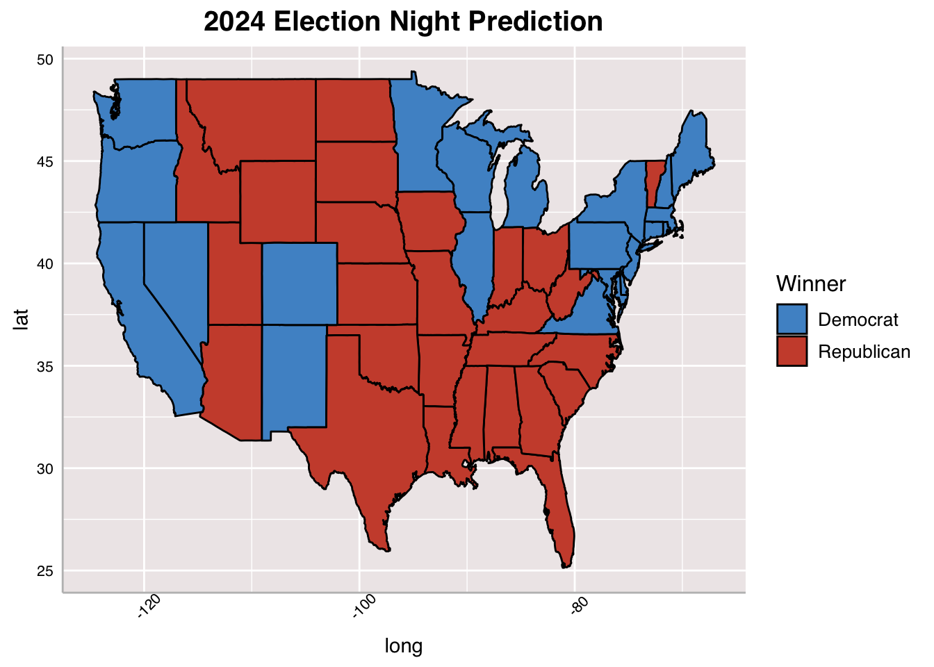
To update this week’s model, I involved campaign expenditure data alongside economic fundamentals and polling data. Campaign expenditure data is taken for Democrats only because the model predicts for Democrats and calculates Republican by subtracting Democratic vote share from 100. The last model individually predicted each party’s vote share, which made it difficult to really see who was ahead.
I, then, regularize the model, using LASSO which is a machine learning model that selects relevant features and neutralizes features that are not. This was helpful to making election results appear more realistic. The final results of this model show an incredibly close race with Harris winning over Trump by just 8 electoral votes. The model forecasts that Trump will take Arizona, Georgia, and North Carolina while Harris takes Pennsylvania, Nevada, and Michigan. This presents a pretty even split among swing states between the two candidates.
Conclusion #
According to this week’s models, Harris will win the 2024 Presidential Election, taking 273 electoral votes.
In comparison to last week’s model, this week presents a much closer race between Harris and Trump, which I believe will be the case. I made an effort to regularize my model this week, which I did not last week, and I think that is mainly why this week’s model presents a much much tighter margin. I will continue to regualarize my models going forward as a result. The involvement of campaign expenditure seems to advantage Democrats in this race, which would make sense considering Harris has raked in $1 billion since entering the race (Goldmacher & Haberman).
Sources #
Goldmacher, Shane and Maggie Haberman. “Harris Raises $1 Billion, Cementing Status as Fundraising Powerhouse.” The New York Times, 9 Oct. 2024, www.nytimes.com/2024/10/09/us/politics/harris-billion-dollar-fundraising.html.
Gelman, Andrew. Why We (Usually) Don’t Have to Worry About Multiple Comparisons. Columbia University, www.stat.columbia.edu/~gelman/research/published/badbayesmain.pdf.
Morris, G. Elliot “How Our Polling Averages Work.” FiveThirtyEight, 18 Aug. 2020, fivethirtyeight.com/methodology/how-our-polling-averages-work/.
Polling Data Provided by GOV 1347: Election Analytics teaching staff (which itself drew from the FiveThirtyEight GitHub)
Economic Data Provided by GOV 1347: Election Analytics teaching staff (which itself drew from the Burueau of Economic Analysia and Federal Reserve Economic Data)